Feature Engineering

After conducting exploratory data analysis (EDA), we gained a deeper understanding of the training dataset. Before diving into feature engineering, we first organize the training dataset into the following format:

<class 'pandas.core.frame.DataFrame'>
RangeIndex: 793751 entries, 0 to 793750
Data columns (total 8 columns):
post_key           793751 non-null object
shared_count       793751 non-null int64
comment_count      793751 non-null int64
like_count         793751 non-null int64
collected_count    793751 non-null int64
weekday            793751 non-null int64
hour               793751 non-null int64
is_trending        793751 non-null int64
dtypes: bool(1), int64(6), object(1)
memory usage: 43.1+ MB

In this section, we will discuss the techniques and models used throughout the data pipeline, including over/undersampling, polynomial transformations, one-hot encoding, and tree-based models.

Info

The training process can be divided into three main stages:

1. Resampling
2. Column Transformation
3. Classification

These stages can be represented as the following Pipeline object:

cachedir = mkdtemp()
pipe = Pipeline(steps=[('resampler', 'passthrough'),
                       # ('columntransformer', 'passthrough'),
                       ('classifier', 'passthrough')],
                memory=cachedir)

For each stage, we experiment with two to three different approaches and several hyperparameter settings to identify the optimal combination.

Handling Imbalanced Datasets (STAGE 1)

In a binary classification problem, an imbalanced dataset refers to a scenario where the target variable (\(y\)) is predominantly of one class (majority) with only a small proportion belonging to the other class (minority).

Training a model on such a dataset without addressing the imbalance often results in a biased model that predicts most samples as the majority class, ignoring valuable information from the minority class.

A potential solution is resampling, which can be categorized into oversampling and undersampling:

• Oversampling: Increases the proportion of minority samples in the dataset.
• Undersampling: Reduces the proportion of majority samples in the dataset.

Both methods help the model pay more attention to minority samples during training. The simplest approach is random sampling, where majority samples are removed, or minority samples are duplicated.

The imblearn library provides implementations for various resampling techniques, including RandomOverSampler and RandomUnderSampler. Additionally, we utilize SMOTE and NearMiss. Below is a brief overview:

SMOTE

SMOTE (Synthetic Minority Oversampling Technique) is an oversampling method that synthesizes new minority samples between existing ones, increasing the proportion of the minority class. The following diagram illustrates this:

Image Source

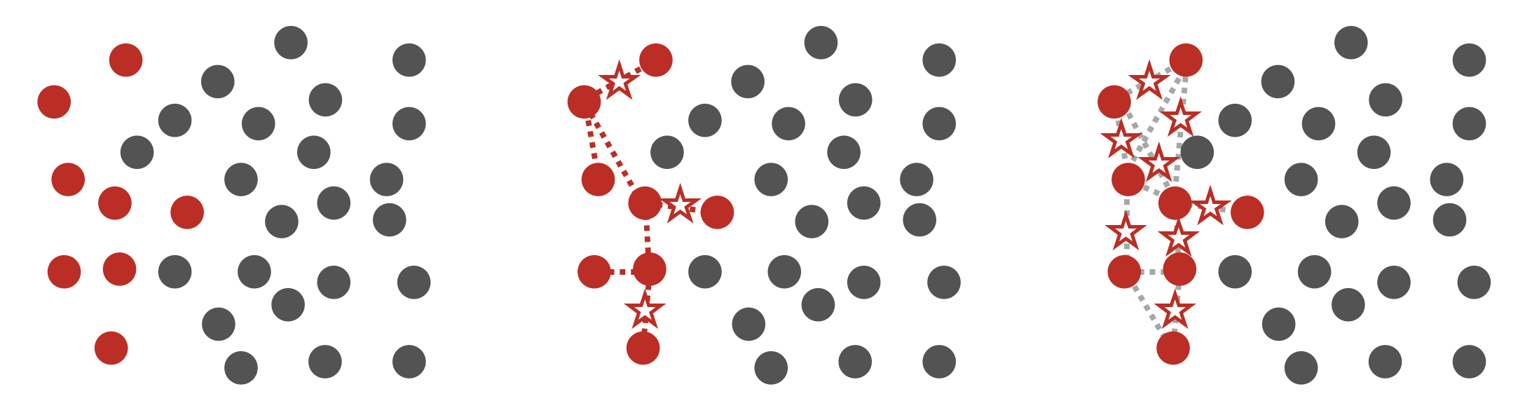
NearMiss

NearMiss is an undersampling method with three versions. We focus on NearMiss-1, which calculates the average distance of all majority samples to their \(k\) nearest minority neighbors and removes the majority samples closest to the minority samples until the class ratio is 1:1. The following diagram illustrates this:

Image Source

Polynomial Transformation and One-hot Encoding (STAGE 2)

Next, we use sklearn's PolynomialFeatures and OneHotEncoder to transform specific features:

• For shared_count, comment_count, liked_count, and collected_count, we apply second-degree polynomial transformations to capture non-linear relationships and interactions between features.
• For the weekday feature, we convert integer values (0 - 6, representing Monday to Sunday) into one-hot encoded vectors, e.g., [1, 0, 0, 0, 0, 0, 0] for Monday.

Tree-based Ensemble Models (STAGE 3)

For classification, we primarily use tree-based ensemble models, including AdaBoostClassifier, GradientBoostingClassifier, and XGBClassifier. These models are chosen for several reasons:

• They are invariant to monotonic transformations of features, reducing the need for extensive feature engineering.
• They offer high interpretability, making it easier to understand feature importance.
• They perform well on large and complex datasets and are often top performers in Kaggle competitions (e.g., XGBoost, LightGBM, CatBoost).

Ensemble learning can be categorized into Bagging (bootstrap aggregating) and Boosting.

Bagging

The most well-known Bagging application is Random Forest, which builds multiple decision trees using bootstrap sampling and random feature selection. Each tree learns a subset of features, and their predictions are aggregated for the final result.

Boosting

Adaptive Boosting

Adaptive Boosting (AdaBoost) sequentially builds \(T\) weak learners \(h_t(x)\), with each model focusing on samples misclassified by the previous one. Each model is assigned a weight \(\alpha_t\) based on its performance:

• Higher weights indicate better performance.
• Lower weights indicate worse performance.

The final model \(H(x)\) aggregates the predictions of all \(T\) weak learners. For more details, refer to this note.

Gradient Boosting

Gradient Boosting builds \(T\) models \(h_t(x)\) sequentially, where each model predicts the gradient (pseudo-residuals) of the previous model's errors. The final model \(H(x)\) is the sum of all previous models. For mathematical derivations, refer to this note.

Extreme Gradient Boosting

XGBoost is an optimized implementation of Gradient Boosting with enhancements like weighted quantile sketch, parallel learning, and cache-aware access. For more details, refer to this paper.

Hyperparameter Optimization

After understanding the techniques used in each stage, we define the possible methods and hyperparameter combinations for each stage as follows:

Resampler - passthrough: No resampling. - NearMiss: Default parameters. - SMOTE: Default parameters.

Column Transformer - passthrough: No feature transformation. - col_trans: Apply polynomial transformations and one-hot encoding.

Classifier - AdaBoostClassifier: Default parameters with tree depth limited to [1, 2, 3]. - GradientBoostingClassifier, XGBClassifier: Default parameters with learning rates [0.025, 0.05, 0.1].

For all classifiers, we set the number of decision trees to [90, 100, 110, 120] and tune additional hyperparameters.

Initially, there are 216 combinations to test, which is too many given time constraints. Experiments show that models with feature transformations generally perform worse, likely due to high feature correlations identified during EDA. As a result, we omit the "Feature Transformation" stage, reducing the combinations to 108. We use GridSearchCV with cv=3 to find the best combination.

The parameter grid is defined as follows:

# poly_cols = ['shared_count', 'comment_count', 'liked_count', 'collected_count']
# col_trans = make_column_transformer((OneHotEncoder(dtype='int'), ['weekday']),
#                                     (PolynomialFeatures(include_bias=False), poly_cols),
#                                     remainder='passthrough')
param_grid_ada = {
    'resampler': ['passthrough', SMOTE(), NearMiss()],
    # 'columntransformer': ['passthrough', col_trans],
    'classifier': [AdaBoostClassifier()],
    'classifier__n_estimators': [90, 100, 110, 120],
    'classifier__base_estimator': [DecisionTreeClassifier(max_depth=1), 
                                   DecisionTreeClassifier(max_depth=2),
                                   DecisionTreeClassifier(max_depth=3)]
}
param_grid_gb = {
    'resampler': ['passthrough', SMOTE(), NearMiss()],
    # 'columntransformer': ['passthrough', col_trans],
    'classifier': [GradientBoostingClassifier(), XGBClassifier()],
    'classifier__n_estimators': [90, 100, 110, 120],
    'classifier__learning_rate': [0.025, 0.05, 0.1]
}
param_grid = [param_grid_ada, param_grid_gb]